The Normal Distribution

Learning Objectives

Understand the properties of the normal distribution and its importance to inferential statistics
Convert a raw score to a z score and vice versa
Familiarize yourself with the standard normal table
Convert a z score into a proportion (or percentage) and vice versa

Key Terms

Normal distribution: a bell-shaped, symmetrical distribution in which the mean, median and mode are all equal
Z scores (also known as standard scores): the number of standard deviations that a given raw score falls above or below the mean
Standard normal distribution: a normal distribution represented in z scores. The standard normal distribution always has a mean of zero and a standard deviation of one.

Overview

What is a distribution? A distribution is an arrangement of values of a variable showing their observed or theoretical frequency of occurrence. A bell curve showing how the class did on our last exam would be an example of a distribution. All distributions can be characterized by the following two dimensions:

1. Central Tendency—what are the mean, median and mode(s) of the distribution?

2. Variability—all distributions have a variance and standard deviation (they also have a range and IQR, but those are less important in inferential statistics).

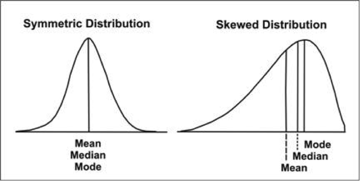
The normal distribution is a bell-shaped, symmetrical distribution in which the mean, median and mode are all equal. If the mean, median and mode are unequal, the distribution will be either positively or negatively skewed. Consider the illustration below:

The Normal Distribution and the Standard Deviation

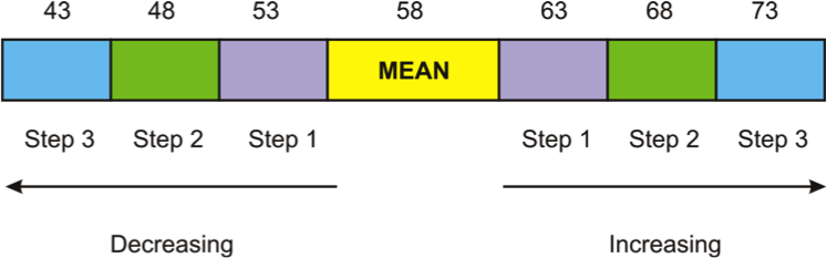
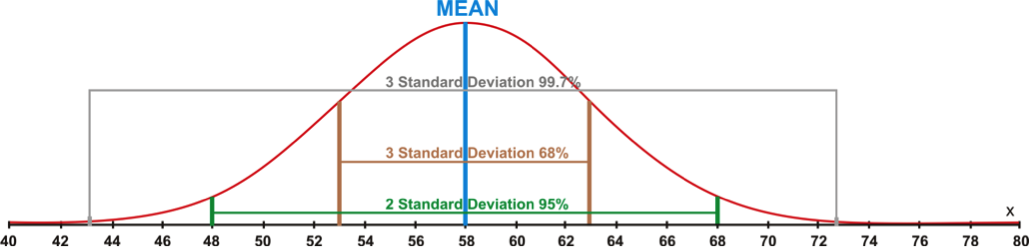
When talking about the normal distribution, it's useful to think of the standard deviation as being steps away from the mean. One step to the right or one step to the left is considered one standard deviation away from the mean. Two steps to the left or two steps to the right are considered two standard deviations away from the mean. Likewise, three steps to the left or three steps to the right are considered three standard deviations from the mean. The standard deviation of a dataset is simply the number (or distance) that constitutes a complete step away from the mean. Adding or subtracting the standard deviation from the mean tells us the scores that constitute a complete step. Below I've put together a distribution with a mean of 58 and a standard deviation of 5. For example, if I add the standard deviation to the mean, I would get a score of 63 (58 + 5 = 63). In stats terminology, we would say that a score of 63 falls exactly "one standard deviation above the mean." Similarly, we could subtract the standard deviation from the mean (58 – 5 = 53) to find the score that falls one standard deviation below the mean.

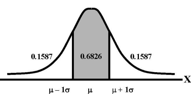
Normal distributions are important due to Chebyshev's Theorem, which states that for a normal distribution a given standard deviation above and/or below the mean will always account for the same amount of area under the curve. Let me explain. Take a look at the picture below. The shaded area represents the total area that falls between one standard deviation above and one standard deviation below the mean. Those Greek letters are just statistical notation for the mean and the standard deviation of a population. Regardless of what a normal distribution looks like or how big or small the standard deviation is, approximately 68 percent of the observations (or 68 percent of the area under the curve) will always fall within two standard deviations (one above and one below) of the mean. Can you guess what proportion falls between the mean and just one standard deviation above it? If you guessed 34, you must be familiar with division (.68/2 = .34).

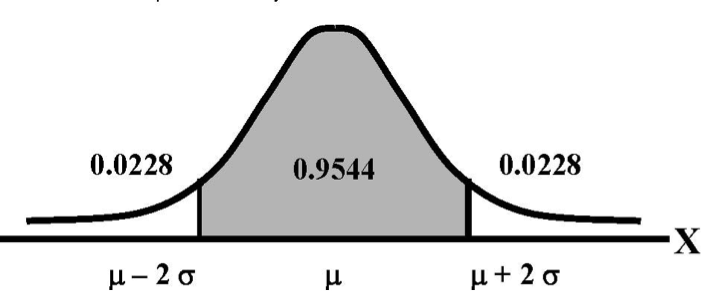
Now take a look at the next picture. It's basically the same as the first instance, only this time we're looking at two standard deviations above and below the mean. For any normal distribution, approximately 95 percent of the observations will fall within this area.

The same thing holds true for our distribution with a mean of 58 and a standard deviation of 5; 68% of the data would be located between 53 and 63. Within this range are all of the data values located within one standard deviation (above or below) of the mean. Furthermore, 95% of the data would fall within two standard deviations of the mean, or in this case between 48 and 68. Finally, 99.7% of the data values would fall between 43 and 73, or within three standard deviations of the mean. The percentages mentioned here make up what some statisticians refer to as the 68%-95%-99.7% rule. These percentages remain the same for all normally distributed data. I've illustrated this principle on the graph below.

Fun fact: the percentage of our distribution that falls in a given area is exactly the same as the probability that any single observation will fall in that area. In other words, we know that approximately 34 percent of our data will fall between the mean and one standard deviation above the mean. We can also say that a given observation has a 34 percent chance of falling between the mean and one standard deviation above the mean. Or, to put it another way, if you were to choose an observation at random from our distribution, there is a 34 percent chance that it would come from the area between the mean and one standard deviation above the mean.

Z Scores

Z scores, which are sometimes called standard scores, represent the number of standard deviations a given raw score is above or below the mean. Sometimes it's helpful to think of z scores as just another unit of measurement. If, for example, we were measuring time, we could express time in terms of seconds, minutes, hours or days. Similarly we could measure distance in terms of inches, feet, yards or miles. We might have to do a little math to convert our data from one unit of measurement to another, but the thing we are measuring remains unchanged.

When we work with z scores, we're basically converting our existing data into a new unit of measurement: standard deviation units. All interval/ratio data can be expressed as z scores. We can convert any raw score into z scores by using the following formula:

In other words, we just need to subtract the mean from the raw score and divide by the standard deviation. Let's go back to our distribution with a mean of 58 and a standard deviation of 5. We can convert 63 (a raw score) into standard deviation units (z scores) fairly easily:

63-58/5 = 5/5 = 1

Just as one hour is equal to 60 minutes, a raw score of 63 in this distribution is equal to one standard deviation. The same holds true for observations below the mean:

53-58/5 = -5/5 = -1

In this case, because our answer is negative, we know that 53 falls exactly one standard deviation below the mean. Now suppose we wanted to convert our mean (58) into a z score:

58-58/5 = 0/5 = 0

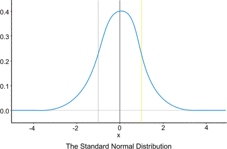
When we convert our data into z scores, the mean will always end up being zero (it is, after all, zero steps away from itself) and the standard deviation will always be one. Data expressed in terms of z scores are known as the standard normal distribution, shown below in all of its glory.

We can also convert z scores back to raw scores with the following formula:

We simply multiply the z score by the standard deviation and add that to the mean. So if we plug the numbers from our example into the formula we get:

Raw score = 58 + 1(5) = 63

Once we've got our heads around the normal distribution, Kuibyshev's theorem and z scores , we can use them to determine the percentage of our data that falls in a given area of our distribution. In order to do that, we need the cumulative z table, which I have posted on Canvas. The cumulative z table tells us what percentage of the distribution falls to the left of a given z score. I know that the table looks pretty intimidating, so we'll spend a significant amount of time going over this in class.

Main Points

The normal distribution is a symmetrical, bell-shaped distribution in which the mean, median and mode are all equal. It is a central component of inferential statistics.
The standard normal distribution is a normal distribution represented in z scores. It always has a mean of zero and a standard deviation of one.
We can use the standard normal table to calculate the area under the curve between any two points

Calculating Z Scores in SPSS

In SPSS, we can compute z scores for any interval/ratio variable via the "Descriptives" command. Click "Analyze," then "Descriptive Statistics," and then "Descriptives." The dialog box for descriptive statistics should pop up. In the bottom-left corner, you will see a check box labeled "Save standardized values as variables." Check this box and move an interval/ratio variable of your choice into the empty box on the right. Then click Okay. At this point, SPSS will calculate a mean for the variable you chose, subtract the value of each case from said mean, then divide the resulting number by the standard deviation of the variable you chose. In the case of the World Values Survey, it will go through that process for all 50,000+ observations. Note: you won't see the z scores listed in the Output window because SPSS inserts them into the Data View window as a new variable (it will likely be labeled Z[insert variable name here]). Congrats! You've just calculated thousands of z scores in the time it would have taken you to calculate one by hand. Here's a video walkthrough:

Exercises

Using the New Immigrant Survey Data, calculate z scores (a.k.a. standardized values) for the "EDUCATION" variable. What is the mean? What is the standard deviation? Now list AND INTERPRET the standardized values for the first five cases. For example, if the standardized value for the first case were -1.75, I might say something like "In terms of educational attainment, this observation falls approximately 1.75 standard deviations below the overall sample mean."
Now repeat the process from Question #1 using the "AGE" variable from the World Values Survey. Again, you must report the mean and the standard deviation before listing and interpreting the standardized values of the first five cases.

The Normal Distribution and Z Scores