Analysis of Variance (ANOVA)
Learning Objectives
- Understand the ANOVA test, its associated assumptions and the context in which it is used.
- Carry out an ANOVA test and interpret the results
- Carry out and interpret a post-hoc test in SPSS
Key Terms
Analysis of variance (ANOVA): a hypothesis test designed to test for a statistically significant difference between
the means of three or more groups
F statistic: the test statistic for ANOVA, calculated as a ratio of the amount of between-group
variation to the amount of within-group variation
Post-hoc test: a test designed to determine which of the group means included in an ANOVA test is
statistically significant from the others
Overview
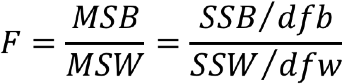
Analysis of variance (ANOVA) is a hypothesis test that is used to compare the means of three or more groups. The logic of ANOVA is very much like the logic of a t test; we might be able to see that sample means are different from one another just by eyeballing them, but we don't know if the difference is statistically significant. In other words, the apparent difference could be due to sampling error. The key difference between ANOVA and a t test is that t tests can only compare two means at a time, while ANOVA has no such restrictions. ANOVA essentially compares the amount of variation between groups with the amount of variation within each group. The result of this comparison is an obtained F statistic, which we must compare to a critical F statistic in order to reach a conclusion. A large F Statistic means that there is more between-group variance than within-group variance, thus increasing our chances of rejecting the null hypothesis. The formula for calculating the F statistic, which we'll deal with in more detail momentarily, looks like this:
When using ANOVA to compare means, our null hypothesis is always that all of the group means are equal. Our research hypothesis, in contrast, is that at least one group mean is different from the others. You should note that ANOVA doesn't tell us which of the group means is different. To figure that out, we need to run a post-hoc test, which is all but impossible to do by hand. We'll talk more about that below.
The following data represent the number of zombies killed by three common household items: a golf club, a baseball bat and a shovel. It sure looks as though there are differences in the number of zombies killed by each weapon, but are these differences due to sampling error, or do they represent real differences in zombie-killing effectiveness? To answer that question, we need to run an ANOVA test.
Number of Zombies Killed by Three Different Weapons
| Golf Club | Baseball Bat | Chainsaw |
| 1 | 4 | 7 |
| 2 | 5 | 8 |
| 3 | 6 | 9 |
As you can see from the formula above, calculating our obtained F statistic requires four major components: the sum of squares between (SSB), the sum of squares within (SSW), the degrees of freedom between (dfb) and the degrees of freedom within (dfw). The following section will walk you through how to calculate each. For the record, calculating ANOVA by hand is a little bit of a process, so now might be a good time to pause for a moment to take a few deep breaths and/or freshen up your cup of coffee.
Step 1) calculate the sum of squares between groups using the following formula:


Where nk = the number of cases in a sample, Yk = the mean of the sample and Y is the overall mean (a.k.a. the "grand mean" or the "mean of means")
Mean of golf club = 2
Mean of baseball bat = 5
Mean of chainsaw = 8
The grand mean (or the mean number of zombies killed overall) is 5. If we plug these numbers into the equation above, we get the following:
3[(2-5)2+(5-5)2+(8-5)2]
3(18) = 54
So the sum of squares between (SSB), which is the first piece of our rather convoluted puzzle, is 54. We'll come back to this momentarily.
Step 2) use the following formula to calculate the sum of squares within groups (SSW):


Where Yi = each individual score in a group and Yk = the mean of that group. For the purposes of this example, this calculation works out as follows:
(1-2)2+(2-2)2+(3-2)2 = 2
(4-5)2+(5-5)2+(6-5)2 = 2
(7-8)2+(8-8)2+(9-8)2 = 2
2 + 2 +2 = 6
The sum of squares within (SSW), which constitutes another piece of our puzzle, is 6. Put a bookmark in this; we'll come back in just a second.
Step 3) calculate the degrees of freedom between groups using the following formula:

In other words, the degrees of freedom between groups is equal to the total number of groups minus one. In this case, the dfb is equal to 3 - 1, or 2.
Step 4) calculate the degrees of freedom within using the following formula:
![]()
The degrees of freedom within groups is equal to N - k, or the total number of observations (9) minus the number of groups (3).
dfw = 9 - 3 = 6
Step 5) calculate the mean squares between groups by dividing the sum of squares between groups (SSB) by the degrees of freedom between groups (dfb). In this example, our SSB is 54 and our dfb is 2, so we find our MSB like so:
54/2 = 27
Step 6) calculate the mean squares within groups by dividing the sum of squares within groups (SSW) by the degrees of freedom within groups (dfw). In this example, our SSW is 6 and our dfw is 6, so the calculations to find the MSW are as follows:
6/6 = 1
Step 7) calculate the F statistic (finally!) by dividing the MSB by the MSW:
27/1 = 27
Our obtained F statistic is 27, which, for the record, is almost comically large. But in order to come to a conclusion, we need to compare it to a critical statistic, which we can find on a table not unlike the one on Canvas. Finding the critical statistic on an F distribution table is a little bit different than either the t distribution table or the chi-square distribution table because this time we actually have two sets of degrees of freedom. The degrees of freedom between groups are found a long the top row, and the degrees of freedom within are found along the leftmost column of the table. The point at which they intersect is the critical statistic we need to come to our conclusion. Because our degrees of freedom are (2,6), we need to go over two columns and down six rows, at which point we encounter our critical statistic of 5.14. Because 27 is greater than 5.14, we can reject the null hypothesis and conclude that at least one group is significantly different from the other two. To determine which group, however, we would need to run a post-hoc test, which we'll talk about in more detail in the video below.
Main Points
- Analysis of variance (ANOVA) is a hypothesis test used to test for statistically significant differences between the means of three or more groups.
- The test statistic for ANOVA is an F statistic. It is essentially a ratio of between-group variation to within-group variation.
- ANOVA tells you whether the mean of at least one group is significantly different from those of the other groups, but it does not tell you which mean.
- In order to determine which mean(s) is/are significantly different from the others, we need to run a post-hoc test. There are several post-hoc tests available for use with ANOVA, but Duncan's is arguably the easiest to interpret in SPSS.
ANOVA Tests in SPSS
To carry out an ANOVA test in SPSS, click on "Analyze," then "Compare Means," and then "One-Way ANOVA." Put the variable for which you want the means tested into the "Dependent List" space and the variable that splits your sample into three or more distinct subgroups in the "Factor" box. Click OK.
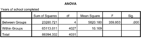
Your output should look something like the screenshot above. The number in the "F" column is your obtained statistic, and the number in the "Sig." column is a p-value that tells whether the F statistic is large enough to conclude that there is a difference in the means of the groups. If that number is less than 0.05, we can conclude that the mean of at least one group is significantly different from the others. Assuming the at least one mean is different from the others, you'll probably want to know which one, which will require a post hoc test. To run a post hoc test, you will need to follow the same steps described above. Click on "Analyze," then "Compare Means," and then "One-Way ANOVA." Make sure the same variables are still in the same boxes, and then click "Post Hoc" and choose the test you would like to perform (I'm a big fan of Duncan's). You can choose whichever you like, but you should only choose one at a time. The results of your post hoc test should look like the screenshot displayed below.
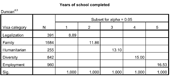
The categories of your "factor" variable are listed in the leftmost column, and the mean for that category is shown in one of the columns to the right. If two categories have their means displayed in the same column, it implies that there is no difference between their means. If the means for two categories are in different columns, it implies that their means are significantly different from one another. For a more detailed explanation of ANOVA and post hoc tests, see this video walkthrough:
SPSS Exercises
- Using the ADD Health data, test for a difference in income by race.
- Using the NIS data, test for a difference in education by visa category.